


Artificial neural networks are computational models which work similar to the functioning of a human nervous system. There are several kinds of artificial neural networks. These type of networks are implemented based on the mathematical operations and a set of parameters required to determine the output. Lets look at some of the neural networks:
1.Feedforward Neural Network – Artificial Neuron:
This neural network is one of the simplest form of ANN, where the data or the input travels in one direction. The data passes through the input nodes and exit on the output nodes. This neural network may or may not have the hidden layers. In simple words, it has a front propagated wave and no back propagation by using a classifying activation function usually.
2.Radial basis function Neural Network:
Radial basic functions consider the distance of a point with respect to the center. RBF functions have two layers, first where the features are combined with the Radial Basis Function in the inner layer and then the output of these features are taken into consideration while computing the same output in the next time-step which is basically a memory. Below is a diagram which represents the distance calculating from the center to a point in the plane similar to a radius of the circle. Here, the distance measure used in euclidean, other distance measures can also be used. The model depends on the maximum reach or the radius of the circle in classifying the points into different categories. If the point is in or around the radius, the likelihood of the new point begin classified into that class is high. There can be a transition while changing from one region to another and this can be controlled by the beta function.
This neural network has been applied in Power Restoration Systems. Power systems have increased in size and complexity. Both factors increase the risk of major power outages. After a blackout, power needs to be restored as quickly and reliably as possible. This paper how RBFnn has been implemented in this domain. Power restoration usually proceeds in the following order: • First priority is to restore power to essential customers in the communities. These customers provide health care and safety services to all and restoring power to them first enables them to help many others. Essential customers include health care facilities, school boards, critical municipal infrastructure, and police and fire services. • Then focus on major power lines and substations that serve larger numbers of customers • Give higher priority to repairs that will get the largest number of customers back in service as quickly as possible • Then restore power to smaller neighborhoods and individual homes and businesses . The diagram below shows the typical order of power restoration system.
Referring to the diagram, first priority goes to fixing the problem at point A, on the transmission line. With this line out, none of the houses can have power restored. Next, fixing the problem at B on the main distribution line running out of the substation. Houses 2, 3, 4 and 5 are affected by this problem. Next, fixing the line at C, affecting houses 4 and 5. Finally, we would fix the service line at D to house 1.
Kohonen Self Organizing Neural Network:
The objective of a Kohonen map is to input vectors of arbitrary dimension to discrete map comprised of neurons. The map needs to me trained to create its own organization of the training data. It comprises of either one or two dimensions. When training the map the location of the neuron remains constant but the weights differ depending on the value. This self organization process has different parts, in the first phase every neuron value is initialized with a small weight and the input vector. In the second phase, the neuron closest to the point is the ‘winning neuron’ and the neurons connected to the winning neuron will also move towards the point like in the graphic below. The distance between the point and the neurons is calculated by the euclidean distance, the neuron with the least distance wins. Through the iterations, all the points are clustered and each neuron represents each kind of cluster. This is the gist behind the organization of Kohonen Neural Network. Image Kohonen Neural Network is used to recognize patterns in the data. Its application can be found in medical analysis to cluster data into different categories. Kohonen map was able to classify patients having glomerular or tubular with an high accuracy.
Recurrent Neural Network(RNN) – Long Short Term Memory:
The Recurrent Neural Network works on the principle of saving the output of a layer and feeding this back to the input to help in predicting the outcome of the layer. Here, the first layer is formed similar to the feed forward neural network with the product of the sum of the weights and the features. The recurrent neural network process starts once this is computed, this means that from one time step to the next each neuron will remember some information it had in the previous time-step. This makes each neuron act like a memory cell in performing computations. In this process, we need to let the neural network to work on the front propagation and remember what information it needs for later use. Here, if the prediction is wrong we use the learning rate or error correction to make small changes so that it will gradually work towards making the right prediction during the back propagation. This is how a basic Recurrent Neural Network looks like,
The application of Recurrent Neural Networks can be found in text to speech(TTS) conversion models. I read this page about RNN and its application, I found it super intersting, I highly recommend you should read it, if you are intersted in knowing more about RNN. I bet you can understand RNN in details after reading this page.
Convolutional Neural Network:
Convolutional neural networks are similar to feed forward neural networks , where the neurons have learn-able weights and biases. Its application have been in signal and image processing which takes over OpenCV in field of computer vision. Below is a representation of a ConvNet, in this neural network, the input features are taken in batch wise like a filter. This will help the network to remember the images in parts and can compute the operations. These computations involve conversion of the image from RGB or HSI scale to Gray-scale. Once we have this, the changes in the pixel value will help detecting the edges and images can be classified into different categories.
ConvNet are applied in techniques like signal processing and image classification techniques. Computer vision techniques are dominated by convolutional neural networks because of their accuracy in image classification. The technique of image analysis and recognition, where the agriculture and weather features are extracted from the open source satellites like LSAT to predict the future growth and yield of a particular land are being implemented. 6.Modular Neural Network: Modular Neural Networks have a collection of different networks working independently and contributing towards the output. Each neural network has a set of inputs which are unique compared to other networks constructing and performing sub-tasks. These networks do not interact or signal each other in accomplishing the tasks. The advantage of a modular neural network is that it breakdowns a large computational process into smaller components decreasing the complexity. This breakdown will help in decreasing the number of connections and negates the interaction of these network with each other, which in turn will increase the computation speed. However, the processing time will depend on the number of neurons and their involvement in computing the results.
Long short-term memory (LSTM)
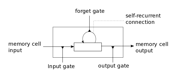
In a traditional recurrent neural network, during the gradient back-propagation phase, the gradient signal can end up being multiplied a large number of times (as many as the number of timesteps) by the weight matrix associated with the connections between the neurons of the recurrent hidden layer. This means that, the magnitude of weights in the transition matrix can have a strong impact on the learning process. If the weights in this matrix are small (or, more formally, if the leading eigenvalue of the weight matrix is smaller than 1.0), it can lead to a situation called vanishing gradients where the gradient signal gets so small that learning either becomes very slow or stops working altogether. It can also make more difficult the task of learning long-term dependencies in the data. Conversely, if the weights in this matrix are large (or, again, more formally, if the leading eigenvalue of the weight matrix is larger than 1.0), it can lead to a situation where the gradient signal is so large that it can cause learning to diverge. This is often referred to as exploding gradients. These issues are the main motivation behind the LSTM model which introduces a new structure called a memory cell (see Figure 1 below). A memory cell is composed of four main elements: an input gate, a neuron with a self-recurrent connection (a connection to itself), a forget gate and an output gate. The self-recurrent connection has a weight of 1.0 and ensures that, barring any outside interference, the state of a memory cell can remain constant from one timestep to another. The gates serve to modulate the interactions between the memory cell itself and its environment. The input gate can allow incoming signal to alter the state of the memory cell or block it. On the other hand, the output gate can allow the state of the memory cell to have an effect on other neurons or prevent it. Finally, the forget gate can modulate the memory cell’s self-recurrent connection, allowing the cell to remember or forget its previous state, as needed.
Multilayer perceptron (MLP)
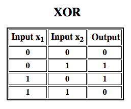
A perceptron is a linear classifier; that is, it is an algorithm that classifies input by separating two categories with a straight line. Input is typically a feature vector x multiplied by weights w and added to a bias b: y = w * x + b. A perceptron produces a single output based on several real-valued inputs by forming a linear combination using its input weights. perceptron uses performing non-linear classification, such as the XOR function.Subsequent work with multilayer perceptrons has shown that they are capable of approximating an XOR operator as well as many other non-linear functions.
A multilayer perceptron (MLP) is a deep, artificial neural network. It is composed of more than one perceptron. They are composed of an input layer to receive the signal, an output layer that makes a decision or prediction about the input, and in between those two, an arbitrary number of hidden layers that are the true computational engine of the MLP. MLPs with one hidden layer are capable of approximating any continuous function. Multilayer perceptrons are often applied to supervised learning problems3: they train on a set of input-output pairs and learn to model the correlation (or dependencies) between those inputs and outputs. Training involves adjusting the parameters, or the weights and biases, of the model in order to minimize error. Backpropagation is used to make those weigh and bias adjustments relative to the error, and the error itself can be measured in a variety of ways, including by root mean squared error (RMSE). Feedforward networks such as MLPs are like tennis, or ping pong. They are mainly involved in two motions, a constant back and forth. You can think of this ping pong of guesses and answers as a kind of accelerated science, since each guess is a test of what we think we know, and each response is feedback letting us know how wrong we are. In the forward pass, the signal flow moves from the input layer through the hidden layers to the output layer, and the decision of the output layer is measured against the ground truth labels. In the backward pass, using backpropagation and the chain rule of calculus, partial derivatives of the error function w.r.t. the various weights and biases are back-propagated through the MLP. That act of differentiation gives us a gradient, or a landscape of error, along which the parameters may be adjusted as they move the MLP one step closer to the error minimum. This can be done with any gradient-based optimisation algorithm such as stochastic gradient descent. The network keeps playing that game of tennis until the error can go no lower. This state is known as convergence.
Refrence:
Comments